- Discrete R.V.에서 Expected Value
(Expected Value는 개별적인 확률 변수의 값들을 나타내는 것이 아니라 그 확률 변수들이 나타내는 전체 분포의 특성을 요약해서 나타내는 요약이다.)
Def)
X가 discrete r.v.이고 m이 X의 distribution func. Ω가 sample space라고 하면
expected value(mean) E(X)은 x*m(x)의 총 합을 의미한다.

만약 x*m(x)의 sum이 수렴하지 않는다면, 기댓값이 무한한 것이 아니라 X는 Expected value가 없다고 표현한다.
ex)
tossing a fair coin 3 times.
r.v. X : # of heads.
Ω = {0,1,2,3}
E(X) = 0*m(0)+1*m(1)+2*m(2)+3*m(3)
= 0*1/8 + 1*3/8 + 2*3/8 + 3*1/8 = 3/2
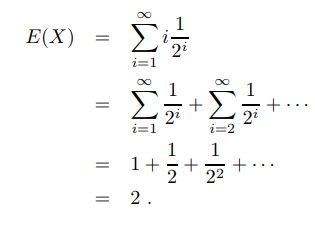
ex)
tossing a fair coin until the first head comes up
r.v. X = # of tosses
Ω={1,2,3,...}
m(i) = 1/(2^i)
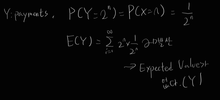
ex)
이전 ex에 이어서 같은 r.v. X에 대해
if X=n. we pay 2^n won. expected payment?
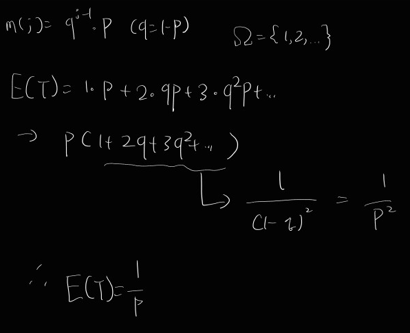
ex)
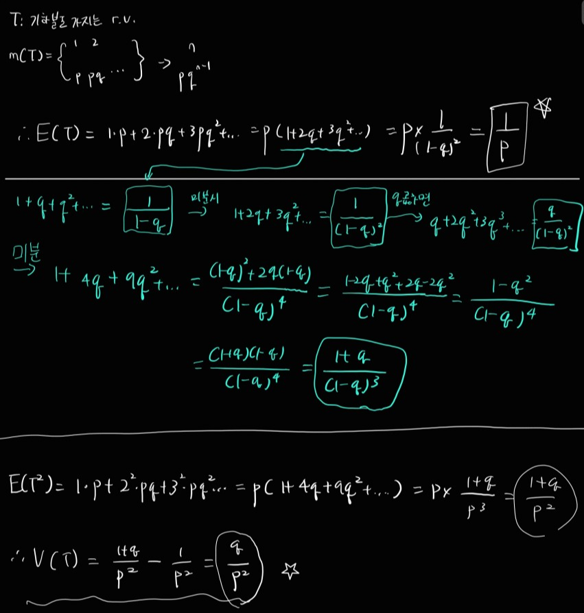
T: time for the 1st success in Bernoulli trial with the parameter p (0<p<1). (T has geometric distribution)
E(T)?
* Expectation of a Function of a Random Variable.
- X가 discrete r.v. with the sample space Ω이며, ϕ가 Ω->R인 function일 시,
E(ϕ(X)) = sum( ϕ(x)m(x)) 이다.
* The sum of the r.v.
X,Y가 expected value를 지니는 r.v.라고 해보자. 그러면 다음의 성질이 성립한다.
i) E(X+Y) = E(X)+E(Y)
ii) E(cX) = cE(X)
즉, E는 linear transformation으로 취급가능하다.
따라서 E(aX+bY+cZ) = aE(X)+bE(Y)+cE(Z) 로 정리 가능하다.
증명)
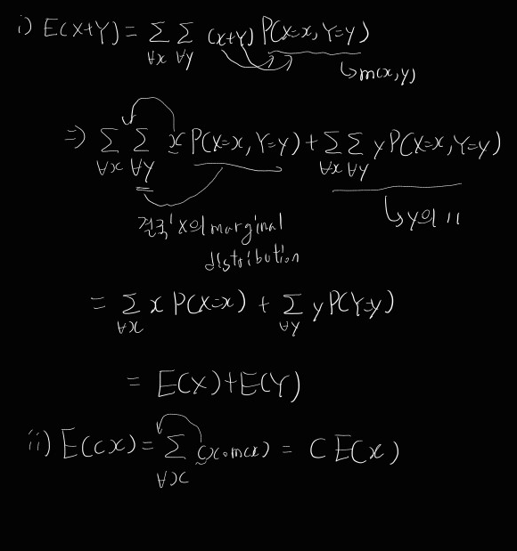
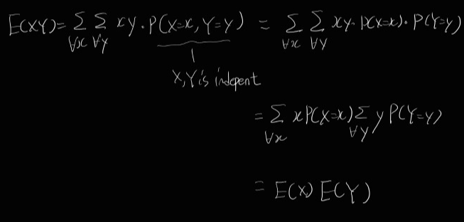
i)을 조금 더 설명하면 결국 y summation 기준 상수항인 x를 밖으로 빼고, P(X=x, Y=y)를 모든 y에 대해 합하면, P(X=x)부분만 남게 된다.
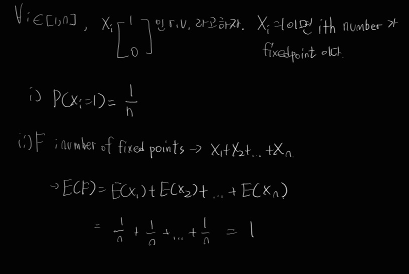
ex)
average number of fixed points in the random permutation.
* Bernoulli trials
- Sn이 number of successes in n Bernoulli trials with prob. p 라면,
E(Sn) = E(X1+X2+X3+...+Xn) = E(X1)+E(X2)+...+E(Xn) = p + p + p + p +... = np
(E(Xi) = 1*p+0*q)
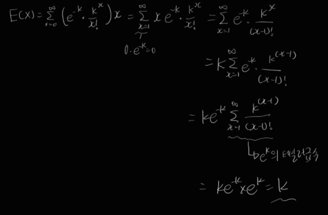
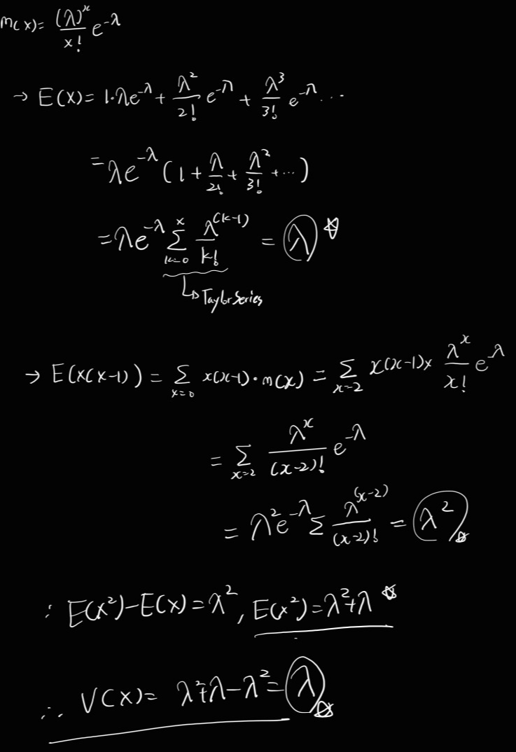
*Poisson distribution
X가 parameter k를 지닌 poisson distribution을 지닌 r.v.이다.
E(X)?
* Independence
만약 X,Y가 independent라면, E(XY) = E(X)E(Y)이다.
증명)
ex)
toss a coin twice
i=1,2.
Xi = 1 (i-th toss is head), 0 (otherwise)
E(X1)=E(X2)= 1*1/2 + 0*1/2 (X1,X2 are independent)
E(X1X2) = E(X1)*E(X2) = 1/4
ex)
toss a coin
X = 1 (head), 0(otherwise)
Y = 1-X
E(X) = 1*1/2 + 0 * 1/2 = 1/2
E(Y) = 0*1/2 + 1*1/2 = 1/2
E(XY) = 0. (xyP(X=x,Y=y)에서 x=1일시 y=0)
X,Y are not independent
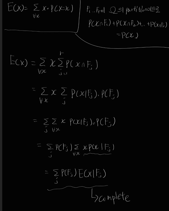
* Conditional Expectation
- F: any event with P(F)>0
X: r.v. with the sample space Ω.

또한, F1...Fr이 sample space의 partition이라면,

증명)
6.2. Variance of Discrete Random Variables
* Variance : 자신의 Expected Value에서 얼마나 값들이 떨어져있나를 설명하는 수치.
Def)
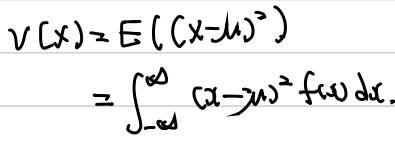
X : μ = E(X)를 expected value로 지니는 r.v. 일 시, X의 variance는 다음과 같이 정의된다.
V(X) = E((x- μ)^2) = sum((x- μ)^2*m(x))
(σ^2)
표준편차 (σ) = sqrt(V(X))이다.
ex)
Roll a die
μ=1/6(1+2+3+...+6)=7/2
V(X) = 1/6(25/4+9/4+1/4+1/4+9/4+25/4) = 35/12
σ = sqrt(35/12) ~= 1.707
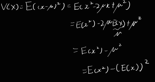
=> 분산 계산 간략화 : V(X)=E(X^2)-((E(X))^2)
증명)
ex)
Roll a die
E(X) = 7/2
E(X^2) = 1/6(1+4+9+16+25+36) = 91/6
V(X) = 91/6 - 49/4 = 35/12
* Properties of Variance
=> X=r.v., c=constant
i) V(cX) = c^2*V(X)
ii) V(X+c) = V(X)
증명)
i) V(cX) = E((cX-E(cX)^2) = E(c^2(X-E(X)^2) = c^2*E((X-E(X))^2) = c^2*V(X)
ii) V(c+X) = E(((X+c) - E(X+c))^2) = E((X-E(X))^2) = V(X)
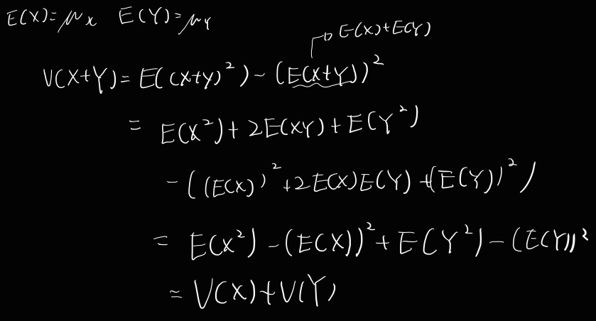
* Thm : X,Y가 독립인 r.v.라면 V(X+Y) = V(X)+V(Y)
증명)
* Thm : X1,...,Xn이 i.i.d를 따르고, E(Xi) = μ, V(Xi) = σ^2 이라고 하자.
만약 r.v. Sn = X1+X2+...+Xm이고 An = Sn/n 이라면,
E(Sn) = nμ, E(An) = μ
V(Sn) = nσ^2, V(An) = V(1/n*Sn) = V(Sn)/n^2 = σ^2/n (따라서 n이 매우 커지면 An 은 분산이 0이 되므로 사실상 μ가 된다.)
* Bernoulli trials(X1 ... Xn)=> r.v. Xj = 1 ( Sucess ), 0 ( Fail )
E(Xj) = 1*p + 0*q = p
E(Xj^2) = 1*p + 0*q = p
V(Xj) = p-p^2 = p(1-p)=pq.
Sn = X1+...+Xn이라고 할 때(Number of Sucess), E(Sn)=np, E(An)=p, V(Sn)=npq, V(An)=pq/n 이다.
Ex)
r.v. T : parameter p를 지니는 Bernoulli 시도에서 첫번째 성공을 할 때까지 시도한 횟수. (기하 분포)
=> T의 variance?
( (f(x)/g(x))' = ( f'(x)g(x) - f(x)g'(x) ) / (g(x))^2 )
Ex)
X가 파라미터 λ를 가지는 Poisson 분포를 따른다 했을 때, Variance?
6.3. Continuous Random Variables Expected Value.
Def)
X가 density function f(x)를 지니는 continuous r.v.일 때, expected value E(X)는 다음과 같다.

즉 이산의 경우 x*m(x)를 전부 더했다면 연속의 경우는 구간 내의 xf(x)를 전부 적분하는 것이다.
Thm)
X,Y가 연속인 r.v.고 c가 constant라면
E(X+Y) = E(X)+E(Y), E(cX) = c*E(X)
Ex)
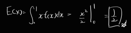
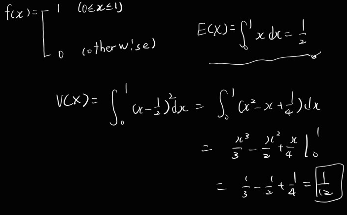
X: 구간 [0,1]에서 uniformly distributed r.v.
f(x) = 1 (0<=x<=1), 0(other). E(X)?
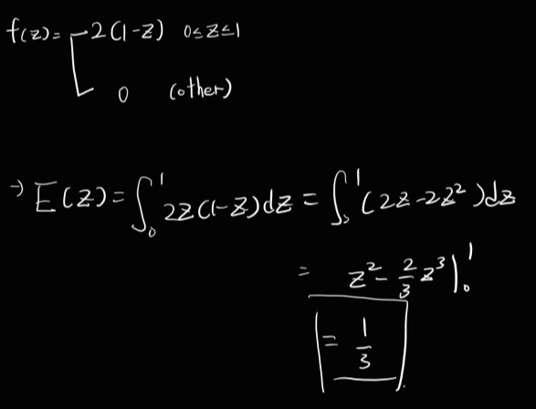
Ex)
Z가 conti r.v.고 f(z) = 2(1-z) (0<=z<=1), 0 (other) 일 시, E(Z)?
Thm)
X가 conti. r.v.이고 Φ : R->R일 때,

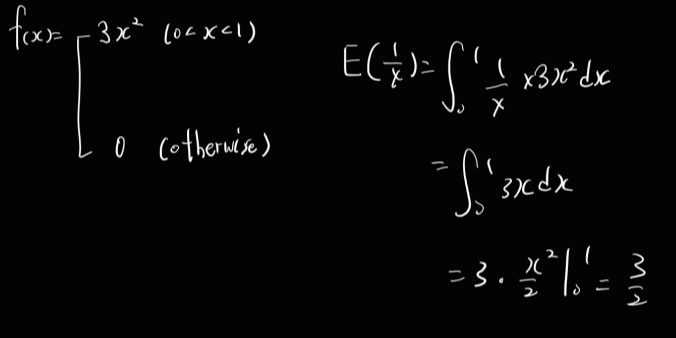
Ex)
X : conti. r.v. with density func. f
f(x) = 3x^2 (0<x<1), 0 (otherwise)
E(1/x)?
Thm)
X,Y가 conti r.v.면서 independent라면
E(XY) = E(X)*E(Y)
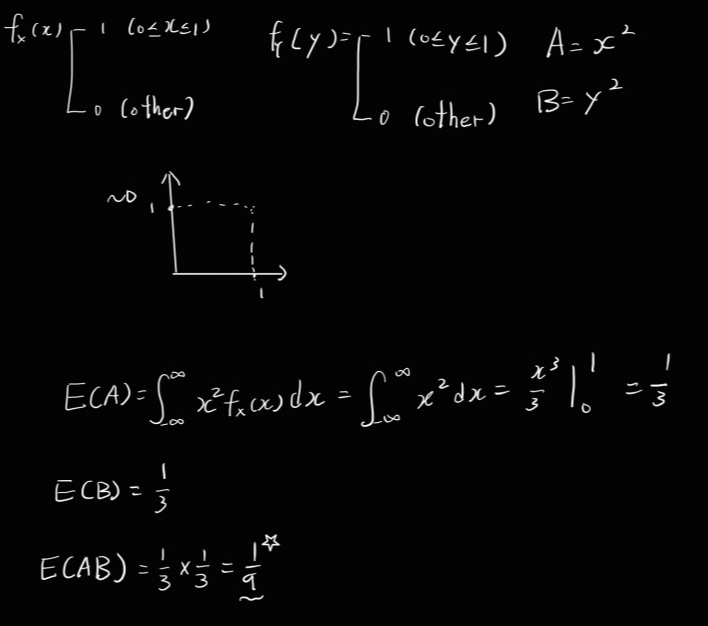
Ex)
r.v. Z = (X,Y), point in the unit square.
fx(x) = 1 (0<=x<=1), 0 (other)
fy(y) = ''
r.v. A = x^2, B = y^2. A,B are independent.
E(AB)?
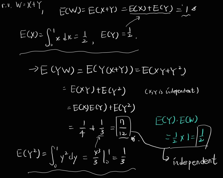
W = X+Y. Y, W are not independent?
* Variance
* Properties of Variance

* X,Y가 independent일 경우
V(X+Y) = V(X)+V(Y)
==> 기본적인 특성은 Discrete와 같다.
Ex)
x: r.v. uniformly distributed on the interval [0,1]
f(x) = 1 (0<=x<=1), 0 (otherwise)
E(X), V(X)?
Ex)
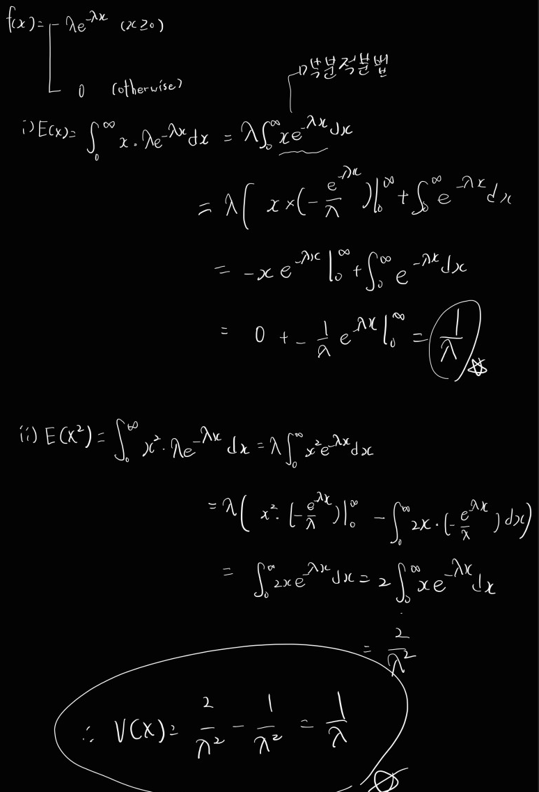
X : esponentially distributed with parameter λ>0.
V(X)?
Ex)
X가 정규분포 따를 때, V(X)?
X가 평균이 μ, 분산이 σ^2인 정규분포를 따를 때, E(X) = μ, V(X) = σ^2 이다.
* Independent trials
-> X1,...,Xn이 conti. r.v., i.i.d이며 E(Xi)= μ, V(Xi)= σ^2 이며 Sn = X1+X2+...+Xn, An = Sn/n 이라고 했을 때
E(Sn) = nμ, E(An)=μ, V(Sn)=n*σ^2, V(An)=σ^2/n
=> 이럴때, Sn을 표준 정규분포로 변환을 시키면
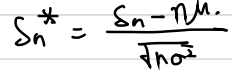
이와 같이 변환시킬 수 있으며, 이렇게 변환된 Sn들은
E(Sn')=0, V(Sn')=1 을 따른다.
'개인 공부' 카테고리의 다른 글
| HCI - Learnability (0) | 2024.04.10 |
|---|---|
| 데이터 과학 - 7. Visualization Theory (0) | 2024.04.10 |
| 데이터 과학 - 6. Data Understanding & Visualization (0) | 2024.04.09 |
| 데이터 과학 - 5. Data Acquisition (0) | 2024.04.09 |
| 데이터 과학 - 4. Data Mining/Science Algorithms (0) | 2024.04.08 |